0.5% Nyquist Imaging via Deep Learning
We present a novel framework for Computational Ghost Imaging based on Deep Learning (CGIDL) and pink noise patterns, which substantially decreases the sampling ratio over 10 times smaller than previous CGIDL work. Here, the deep neural network, which can learn the sensing model and increase the quality image reconstruction, is trained only by simulation results. There is no necessity to conduct experiments to get training inputs (non-experimental) and add noise to customize with a real imaging system (noise-free). This one-time trained network can be applied to multiple environments and various situations. To demonstrate our sub-Nyquist achievement level, a group of detailed comparisons between conventional Computational Ghost Imaging results, imaging results reconstructed using pink noise and white noise via Deep Learning are shown in several sampling levels rate. To indicate its non-experimental advantage, a group of results with strong environmental noise is presented as well. This method has great poten- tials in various applications that require a low sampling rate, quick reconstruction efficiency, and strong turbulence.
Our work based on pink noise patterns and Deep Learning method. There are some work focusing on the CGIDL. However, we have to pay attention that most of them use numerous experiments to get the training deep neutral network because they have to let the network be accustomed to the environmental noise. Otherwise, the Deep Learning process cannot make amelioration on the CGI results (even make it worse). Therefore, the training process tends to be complicated and time consuming. In addition, most work just reach to 5% Nyquist limit in CGI system. On the other hand, the work based on simulational trainings cannot reach that much low rate of Nyquist limit (mostly over 10% Nyquist limit).
Our former work has already proved that the pink noise can realize the noise-free imaging, which means the results of CGI with pink noise patterns usually have less differences between experiments and simulations. Our former work based orthonormal method demonstrates the other advantage of pink noise as well (sub-Nyquist). Thus, it is not hard to believe that the deep learning and pink noise patterns can be combined and reach to extremely low sampling ratio with non-experimental training. This one-time training ought to be noise-free.

Fig. 1. The flow chart of CGIDL. The DNN model is trained in the training process (in red), and test images are for the testing stage (in orange). The experiment process is on the left bottom functioned as the input of trained DNN, and the experimental DL process is on the right bottom side (in purple).
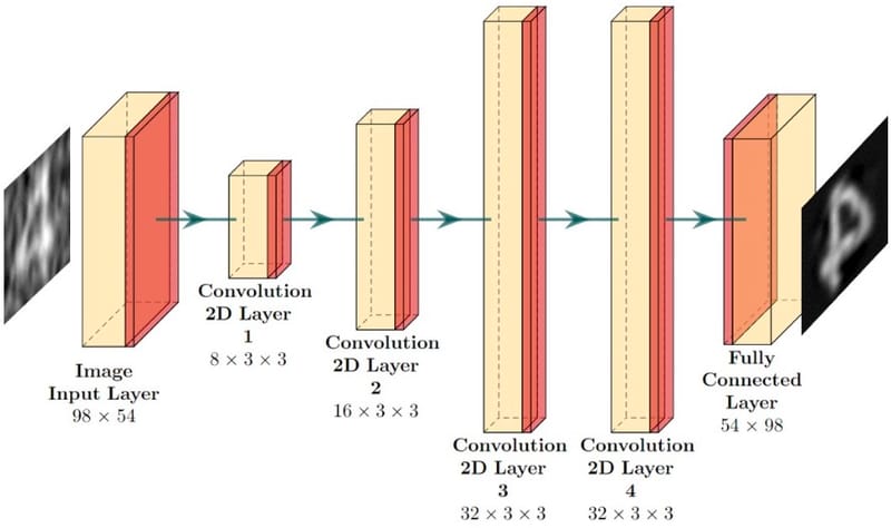
The proposed scheme, as shown in Fig. 1, is a two-step process to reconstruct the CGIDL. Firstly, we construct a network frame-work which is going to be trained later. Specifically, we used a DNN model with four convolution layers, one image input layer, and one image output layer. Small 3 × 3 receptive fields were applied throughout the whole convolution layers which have been proved to perform better by GoogLeNet.The Rec- tified Linear Unit (ReLU) layer and Batch Normalization Layer (BNL) were added between each convolution layer. The BNL is functioned to avoid internal covariate shift during the training process and speeds up the training of DNN. The ReLU layer applies a threshold operation to each element of the inputs. To customize the size of training pictures, both the input and output layers were set as 54 × 98. The solver for training is employed by the Stochastic Gradient Descent with Momentum Optimizer, thus reducing the oscillation via using momentum. Two strategies were applied to avoid over-fitting of training images. At the end of DNN, a dropout layer is aimed to reduce the connection between convo- lution layers and fully connected layer. Meanwhile, learning rate dropped from 0.001 to 0.0001 after 75 epochs, which con- strain the fitting parameters. After the establishment of DNN, plenty of training images are reconstructed by the CGI algorithm, as is mentioned above. Then the training images and reconstruction training images feed the DNN model as inputs and outputs, respectively. Here we use a set of 10000 handwrit- ten digits of 28 × 28 pixels in size from the MNIST handwritten digit database as training images. Compared to the origi- nal training images, we resize images from 28 × 28 to 54 × 98 and normalize them to test a smaller sampling ratio. The maxi- mum epochs were set as 600, and the training iteration is 46800. The program was implemented via MATLAB R2019a Update 5 (9.6.0.1174912, 64-bit), and the DNN was implemented through Deep Learning Toolbox. The GPU-chip NVIDIA GTX1050 was used to accelerate the speed of the computation.
I. Simulation Results
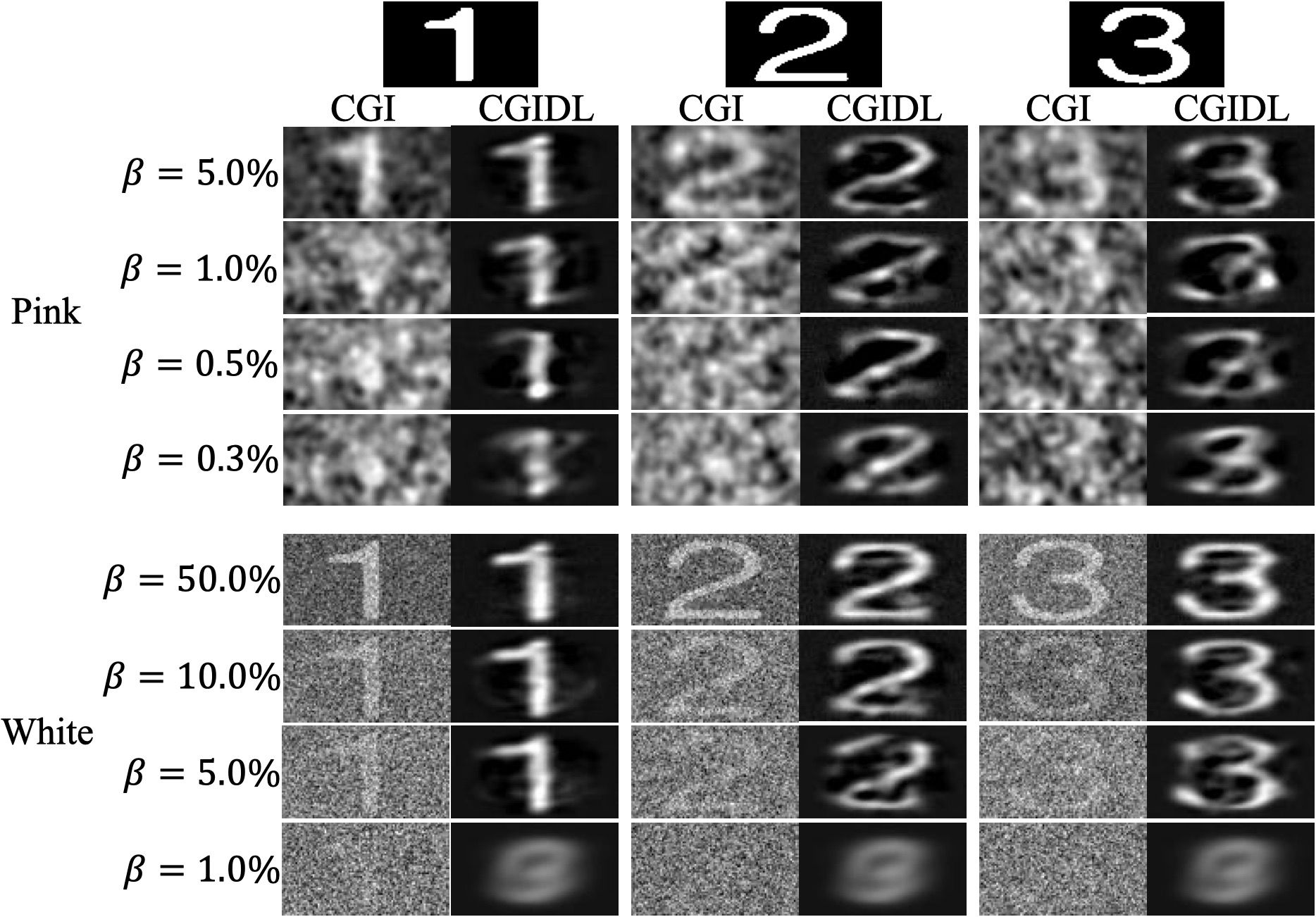
Fig. 2. Main simulation results. For pink noise, we select β = 0.05, 0.01, 0.005, 0.003. However, for white noise when β equals to these small values, the results are totally smeared both under CGI and CGIDL. Thus, here we present β = 0.5, 0.1, 0.05, 0.01 for white noise to make comparison.
II. Experimental Results and Analysis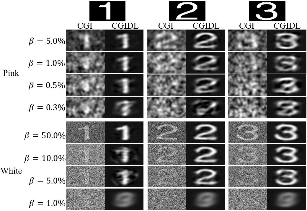
Fig. 3. Main experimental results with 14.68dB noise level. For pink noise, we select β = 0.05, 0.01, 0.005, 0.003. However, for white noise when β equals to these small values, the results are totally smeared both under CGI and CGIDL. Thus, here we present β = 0.5, 0.1, 0.05, 0.01 for white noise to make comparison.
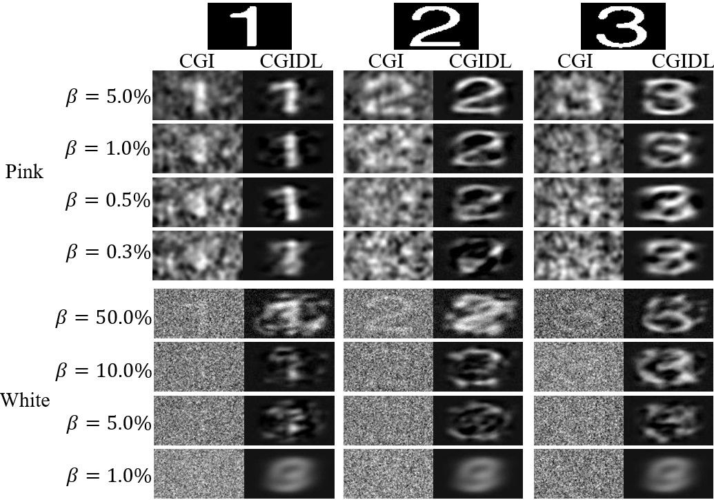 Fig. 4. Main experimental results with 14.68dB noise level. For pink noise, we select β = 0.05, 0.01, 0.005, 0.003. However, for white noise when β equals to these small values, the results are totally smeared both under CGI and CGIDL. Thus, here we present β = 0.5, 0.1, 0.05, 0.01 for white noise to make comparison.
Meanwhile, we also calculate the Mean Square Error (MSE) to justify the quality of the reconstructed image by CGI and CGIDL with pink and white noise, respectively. The Fig. 5. and Fig. 6. present the MSE corresponding to Fig. 3. and Fig. 4.
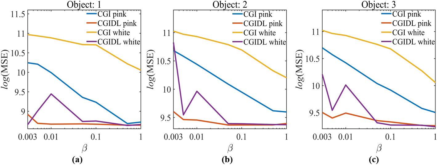
Fig. 5. The MSE of object (a): 1, (b): 2, and (c): 3 in the experiment with noise level at 14.90dB.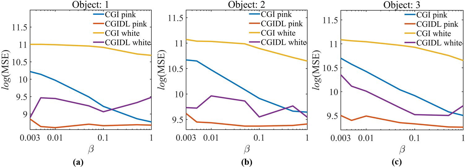
Fig. 6. The MSE of object (a): 1, (b): 2, and (c): 3 in the experiment with noise level at 4.77dB.
To find more detials, please read the manuscript attached below.
